[ ]:
# Author : Dr. Davis Thomas Daniel
# Last updated : 03.09.2025
Data (1D)
Importing EPRpy
[1]:
import eprpy as epr
Loading data
[2]:
tempo = epr.load('tempo.DSC')
[3]:
fig,ax=tempo.plot()
[4]:
type(tempo) # tempo is an EprData object
[4]:
eprpy.loader.EprData
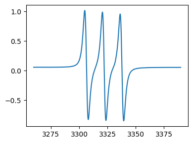
Plotting
Every
EprDataobject has a plot method for making quick plots for inspection.
[5]:
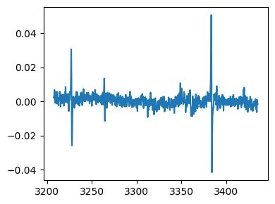
fig,ax = tempo.plot()

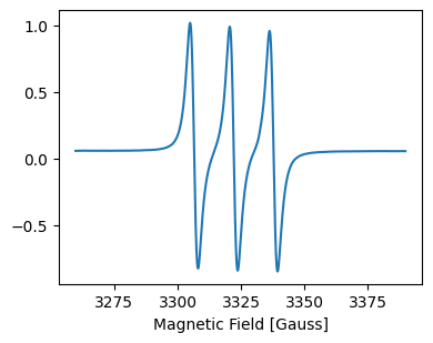
Formatting plots
[6]:
ax.set_xlabel('Magnetic Field [Gauss]') # set x axis label
fig
[6]:
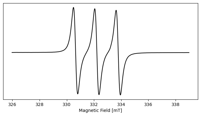
Use attributes directly to plot
Alternatively, plots can be made directly using matplotlib and
EprDataattributes with full control over formatting.
[7]:
import matplotlib.pyplot as plt
fig,ax = plt.subplots(figsize=(8,4))
ax.plot(tempo.x/10,tempo.data,color='black') # convert Gauss to mT
ax.set_xlabel('Magnetic Field [mT]') # set x axis label
_=ax.set_yticks([]) # hide intensity
Plot on the g axis
If the one of the axis is magnetic field, the g values are calculated internally and can be used for plotting as shown below.
[8]:
fig,ax = tempo.plot(g_scale=True)
Operations on Data
Scaling data
[9]:
# import EPRpy
import eprpy as epr
# load data
tempo = epr.load('tempo.DSC')
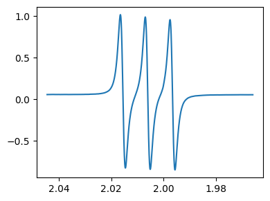
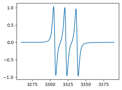
# scale between -1 and 1
tempo_scaled = tempo.scale_between(-1,1)
print('After scaling : ')
fig,ax = tempo_scaled.plot()
After scaling :
Baseline correction
[12]:
# import EPRpy
import eprpy as epr
# load data
tempo = epr.load('tempo.DSC')
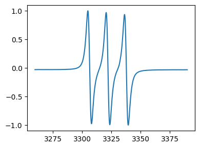
# linear baseline correction
tempo_bc = tempo.baseline_correct(npts=10) # default is linear baseline correction, npts is the data points used for baseline correction, here 10 points from the start and end of data
fig,ax = tempo_bc.plot()
Interactive baseline correction
[19]:
# import EPRpy
import eprpy as epr

# load data needs baseline correction
epr_data = epr.load('data_for_bc.DTA')

# plot the data without bc
fig,ax  = epr_data.plot()
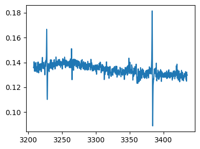
As an example, we baseline correct the spectrum by using a 3° polynomial. For baseline calculation, the points are picked interactively.
[20]:
# if you are using a jupyter notebook, switch to qt backend for matplotlib
#%matplotlib qt

# to switch back to inline mode:
#%matplotlib inline
[ ]:
epr_data_bc = epr_data.baseline_correct(interactive=True, method='polynomial',order=3)
[22]:
# plot the baseline corrected spectra
fig,ax = epr_data_bc.plot()
Computing integrals
[24]:
# import EPRpy
import eprpy as epr

# load data
tempo = epr.load('tempo.DSC')

# baseline correction and integration
tempo_proc = tempo.baseline_correct(npts=10)
tempo_proc = tempo_proc.integral()

# plot the absorption signal
fig,ax = tempo_proc.plot()
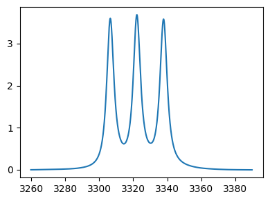
Selecting a region
For this example, we assume that the desired region is the low field hyperfine line.
[25]:
# import EPRpy
import eprpy as epr

# load data
tempo = epr.load('tempo.DSC')

# Plot the data using an array with unity spacing to find corresponding indices
import matplotlib.pyplot as plt
print('Full spectrum : ')
_=plt.plot(tempo.data)

# make a new EprData object corresponding to the desired region
tempo_region = tempo.select_region(range(550,850)) # indices from 0 to 900
Full spectrum :
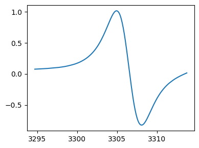
[26]:
# selected region, note that the the new EprData object tempo_region only has the data corresponding to this region
print('Selected region : ')
fig,ax = tempo_region.plot()
Selected region :

History of data operations
EPRpy allows for keeping a log of data operations done on an EprData object, as long as in-built functions are used.
[27]:
# import EPRpy
import eprpy as epr

# load data
tempo = epr.load('tempo.DSC')

# do some operations
tempo_proc1 = tempo.scale_between(-1,1)
tempo_proc2 = tempo_proc1.baseline_correct(npts=10)
tempo_proc3 = tempo_proc2.integral()
Access history
Each
EprDataobject stores history of all data operations and the correspondingEprDataobject in a list of lists. The first item in each list is the description of the data operation and the second item is the correspondingEprDataobject.
[28]:
tempo_proc3.history
[28]:
[['2025-09-03 17:07:52.029357 : Data loaded from tempo.DSC.',
  <eprpy.loader.EprData at 0x13eee9b50>],
 ['2025-09-03 17:07:52.030758 : Data scaled between -1 and 1.',
  <eprpy.loader.EprData at 0x13eee9c40>],
 ['2025-09-03 17:07:52.032316 : Baseline corrected',
  <eprpy.loader.EprData at 0x13eee9ca0>],
 ['2025-09-03 17:07:52.034752 : Integral calculated',
  <eprpy.loader.EprData at 0x13eed4110>]]
To plot or access a specific
EprDatafrom the history, simply use indexing. For instance, to view the original data again, plot the first item in history:
[29]:
print(tempo_proc3.history[0][0])
fig,ax = tempo_proc3.history[0][1].plot()
2025-09-03 17:07:52.029357 : Data loaded from tempo.DSC.
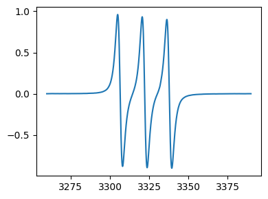
[30]:
print(tempo_proc3.history[2][0])
fig,ax = tempo_proc3.history[2][1].plot()
2025-09-03 17:07:52.032316 : Baseline corrected

Data (2D)
## Importing EPRpy
[31]:
import eprpy as epr
Loading data
[32]:
## TEMPO radical monitored as a function of time
## For some 2D datasets, a .GF file must also be present in the same folder.
tempo2d = epr.load('tempo_time.DSC')
[33]:
tempo2d.data.shape # this dataset corresponds to 48 time values (tempo2d.y) and 1024 field points (tempo2d.x)
[33]:
(48, 1024)
[34]:
tempo2d.y # time in seconds
[34]:
array([    0.  ,  1533.1 ,  3065.64,  4598.25,  6130.95,  7663.46,
        9196.02, 10728.54, 12261.1 , 13793.49, 15326.14, 16858.79,
       18391.58, 19924.32, 21457.01, 22989.5 , 24521.66, 26054.41,
       27586.94, 29119.64, 30652.35, 32184.94, 33717.75, 35250.49,
       36783.1 , 38315.81, 39848.56, 41381.3 , 42913.97, 44446.53,
       45978.94, 47511.65, 49044.47, 50576.93, 52109.66, 53642.3 ,
       55175.05, 56707.73, 58240.42, 59773.14, 61305.37, 62837.76,
       64370.26, 65902.73, 67435.12, 68967.26, 70499.68, 72031.99],
      dtype='>f8')
[35]:
tempo2d.x # field values in Gauss
[35]:
array([3273.65      , 3273.74658203, 3273.84316406, ..., 3372.26025394,
       3372.35683597, 3372.453418  ], shape=(1024,))
Plotting
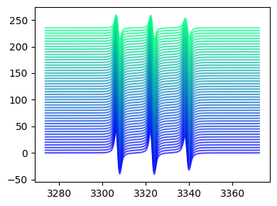
Stacked plot
[36]:
fig,ax = tempo2d.plot(spacing=5)
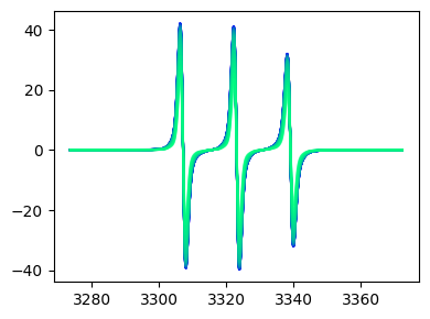
Superimposed plot
[37]:
fig,ax = tempo2d.plot(plot_type='superimposed')
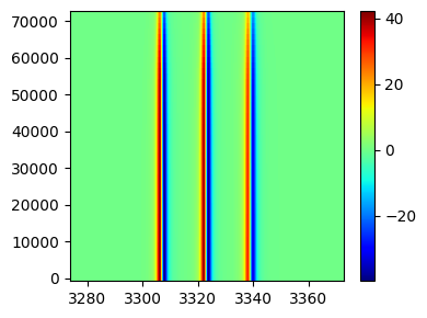
Pseudocolor plots
[38]:
fig,ax = tempo2d.plot(plot_type='pcolor')
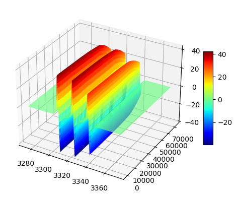
Surface 3D plot
[39]:
fig,ax = tempo2d.plot(plot_type='surf')
Workflows
HYSCORE
[1]:
import eprpy as epr
[2]:
tempo_hyscore = epr.load("tempo_hyscore.DSC")
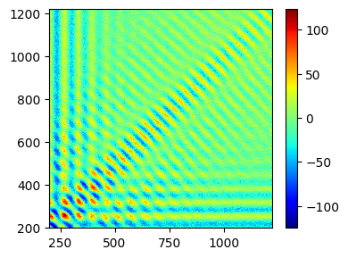
Plot the time-domain data
[3]:
_=tempo_hyscore.plot(plot_type="pcolor")
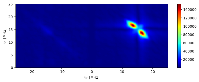
Process using HYSCORE workflow
[4]:
hyscore_proc = tempo_hyscore.workflow(zf=1024) # zero fill with 1024 points
[5]:
fig,ax=hyscore_proc.plot(plot_type="pcolor")
fig.set_size_inches((10,3))
ax.set_ylim((0,25))
ax.set_xlim((-25,25))
ax.set_xlabel(r"$\nu_{2}$"+" [MHz]")
_=ax.set_ylabel(r"$\nu_{1}$"+" [MHz]")
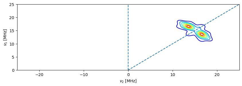
[6]:
# Processing workflows can be controlled by other parameters
# zero fill with 1024 points
# symmetrise the final spectrum along the diagonal
# change polynomila order for background correction to 4
# verbose=True for printing progress

hyscore_proc1 = tempo_hyscore.workflow(zf=1024,symmetrise="diag",poly_order=4,verbose=True)
Starting HYSCORE workflow...
Baseline correction in dimension 1 with polynomial of order 4...
Baseline correction in dimension 2 with polynomial of order 4...
Applying Hamming window in dimension 1...
Applying Hamming window in dimension 2...
Zero filling 1024 points dimension 1 and 2...
Generating frequency axes...
2D Fourier transformation...
Symmetrising along the diagonal and the antidiagonal...
Completed in 0.12 seconds.
[7]:
# you can also plot manually using matplotlib and format to your liking

import matplotlib.pyplot as plt
fig,ax = plt.subplots(figsize=(10,3))
ax.contour(hyscore_proc1.data_dict["frequency_axis1"],hyscore_proc1.data_dict["frequency_axis2"],hyscore_proc1.data,cmap="jet")
ax.set_ylim((0,25))
ax.set_xlim((-25,25))
ax.vlines(0,ymax=25,ymin=0,linestyles="dashed")
ax.plot(hyscore_proc1.x,hyscore_proc1.x,linestyle="dashed")
ax.set_xlabel(r"$\nu_{2}$"+" [MHz]")
_=ax.set_ylabel(r"$\nu_{1}$"+" [MHz]")
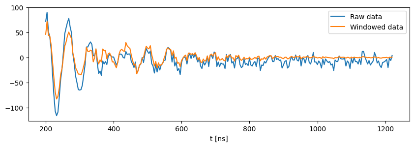
[8]:
# you can also plot other arrays from any step of the processing pipeline
# here the raw time domain data before and after applying a window function is visualized

import matplotlib.pyplot as plt
fig,ax = plt.subplots(figsize=(10,3))

ax.plot(hyscore_proc1.data_dict["x_raw"],hyscore_proc1.data_dict["raw_data"].real[0],label="Raw data")
ax.plot(hyscore_proc1.data_dict["x_raw"],hyscore_proc1.data_dict["bc_w_data"][0],label="Windowed data")
ax.set_xlabel("t [ns]")
_=ax.legend()
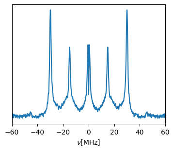
2P ESEEM
[9]:
tempo_eseem = epr.load("tempo_eseem.DSC")
[10]:
_=tempo_eseem.plot()
[11]:
tempo_eseem.pulse_program # this pulse program is supported, check the documentation for pulse programs which support worklfows
[11]:
'2P ESEEM'
[12]:
eseem_proc = tempo_eseem.workflow(zf=1024,verbose=True)
Starting ESEEM workflow...
Detected pulse program : 2P ESEEM
Baseline correction using an exponential decay function...
Applying Hamming window along dimension 1...
Zero filling 1024 points...
Generating frequency axes...
Fourier transformation...
Completed in 0.01 seconds.
[13]:
fig,ax = eseem_proc.plot()
ax.set_xlabel(r"$\nu$" + "[MHz]")
ax.set_xlim((-60,60))
_=ax.set_yticks([])